Black Box Machine Learning
1 Classification algorithms
There is a lot of classification algorithms available now but it is not possible to conclude which one is superior to other. It depends on the application and nature of available data set. For example, if the classes are linearly separable, the linear classifiers like Logistic regression, Fisher’s linear discriminant can outperform sophisticated models and vice versa.
1.1 Decision Tree
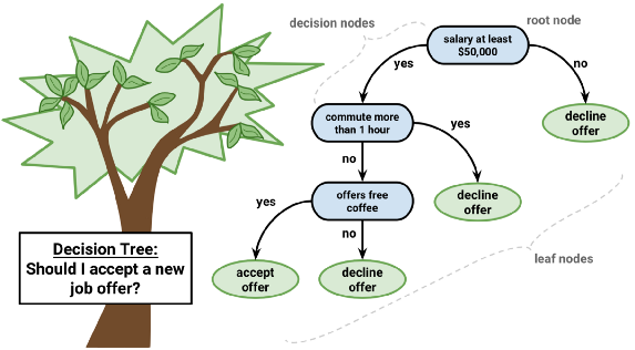
Decision tree builds classification or regression models in the form of a tree structure. It utilizes an if-then rule set. The rules are learned sequentially using the training data one at a time. Each time a rule is learned, the tuples covered by the rules are removed. This process is continued on the training set until meeting a termination condition.
The tree is constructed in a top-down recursive divide-and-conquer manner. All the attributes should be categorical. Otherwise, they should be discretized in advance? Attributes in the top of the tree have more impact towards in the classification and they are identified using the information gain concept.
A decision tree can be easily over-fitted generating too many branches and may reflect anomalies due to noise or outliers. An over-fitted model has a very poor performance on the unseen data even though it gives an impressive performance on training data.
This can be avoided by pre-pruning which halts tree construction early or post-pruning which removes branches from the fully grown tree. What?
1.2 Naive Bayes
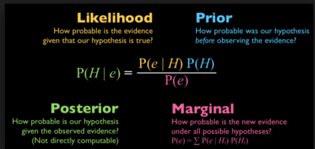
Naive Bayes is a probabilistic classifier inspired by the Bayes theorem under a simple assumption which is the attributes are conditionally independent.
Naive Bayes is a very simple algorithm to implement and good results have obtained in most cases. It can be easily scalable to larger datasets since it takes linear time, rather than by expensive iterative approximation as used for many other types of classifiers.
Naive Bayes can suffer from a problem called the zero probability problem. When the conditional probability is zero for a particular attribute, it fails to give a valid prediction. This needs to be fixed explicitly using a Laplacian estimator?.
1.3 Artificial Neuraul Networks
Artificial Neural Network is a set of connected input/output units where each connection has a weight associated. During the learning phase, the network learns by adjusting the weights so as to be able to predict the correct class label of the input tuples.
There are many network architectures available:
- Feed-forward
- Convolutional
- Recurrent
There can be multiple hidden layers in the model depending on the complexity of the function which is going to be mapped by the model. Having more hidden layers will enable to model complex relationships such as deep neural networks.
However, when there are many hidden layers, it takes a lot of time to train and adjust wights. The other disadvantage of is the poor interpretability of model compared to other models like Decision Trees due to the unknown symbolic meaning behind the learned weights.
But Artificial Neural Networks have performed impressively in most of the real world applications. It has high tolerance to noisy data and is able to classify untrained patterns. Usually, Artificial Neural Networks perform better with continuous-valued inputs and outputs.
All of the above algorithms are eager learners since they train a model in advance to generalize the training data and use it for prediction later.
1.4 k-Nearest Neighbor (KNN)
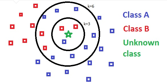
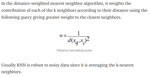
k-Nearest Neighbor is a lazy learning algorithm which stores all instances correspond to training data points in n-dimensional space. When an unknown discrete data is received, it analyzes the closest k number of instances saved (nearest neighbors)and returns the most common class as the prediction and for real-valued data it returns the mean of k nearest neighbors.
nice
2 Evaluating a classifier
After training the model the most important part is to evaluate the classifier to verify its applicability
2.1 Holdout method
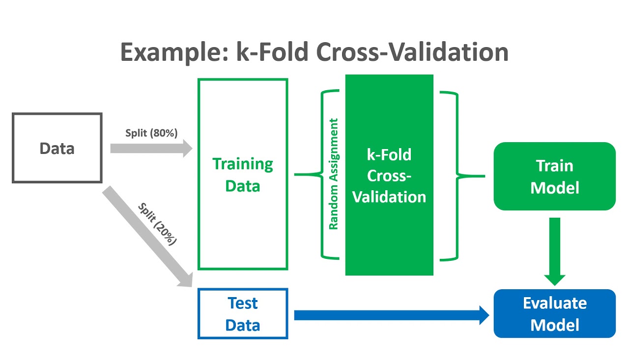
There are several methods exists and the most common method is the holdout method. In this method, the given data set is divided into 2 partitions as test and train 20% and 80% respectively. The train set will be used to train the model and the unseen test data(aaaa, unseen data, I see now) will be used to test its predictive power.
2.2 Cross-validation
Over-fitting is a common problem in machine learning which can occur in most models. k-fold cross-validation can be conducted to verify that the model is not over-fitted. In this method, the data-set is randomly partitioned into k mutually exclusive subsets, each approximately equal size and one is kept for testing while others are used for training. This process is iterated throughout the whole k folds.Sorry what?
2.3 Precision and Recall
Precision is the fraction of relevant instances among the retrieved instances, while recall is the fraction of relevant instances that have been retrieved over the total amount of relevant instances. Precision and Recall are used as a measurement of the relevance.Hmmm…
2.4 ROC curve Receiver Operatning Characteristics
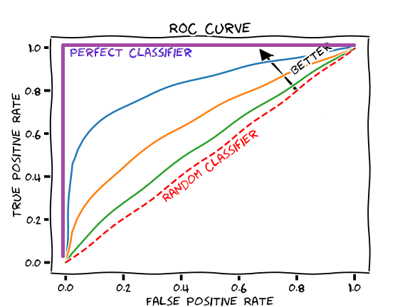
ROC curve is used for visual comparison of classification models which shows the trade-off between the true positive rate and the false positive rate. The area under the ROC curve is a measure of the accuracy of the model. When a model is closer to the diagonal, it is less accurate and the model with perfect accuracy will have an area of 1.0
Alright enough machine lern…oh wait, there are more things to get familiar with in my curriculum.
3 SVM (Support Vector Machine)
Support vector machine is highly preferred by many as it produces significant accuracy with less computation power. Support Vector Machine can be used for both regression and classification tasks. But, it is widely used in classification objectives.
The objective of the support vector machine algorithm is to find a hyperplane in an N-dimensional space(N — the number of features) that distinctly classifies the data points.
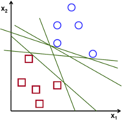
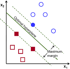
To separate the two classes of data points, there are many possible hyperplanes that could be chosen. Our objective is to find a plane that has the maximum margin, i.e the maximum distance between data points of both classes. Maximizing the margin distance provides some reinforcement so that future data points can be classified with more confidence.
3.1 Hyperplanes and Support Vectors
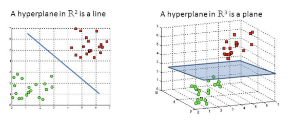
Hyperplanes are decision boundaries that help classify the data points. Data points falling on either side of the hyperplane can be attributed to different classes. Also, the dimension of the hyperplane depends upon the number of features. If the number of input features is 2, then the hyperplane is just a line. If the number of input features is 3, then the hyperplane becomes a two-dimensional plane. It becomes difficult to imagine when the number of features exceeds 3.
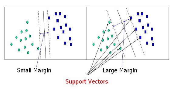
Support vectors are data points that are closer to the hyperplane and influence the position and orientation of the hyperplane. Using these support vectors, we maximize the margin of the classifier. Deleting the support vectors will change the position of the hyperplane. These are the points that help us build our SVM.

Cool, that's a first gif on this website. As easy to put it in as an image, cool. Don't really use them, but why not, I might start to
3.2 Logistic Regression
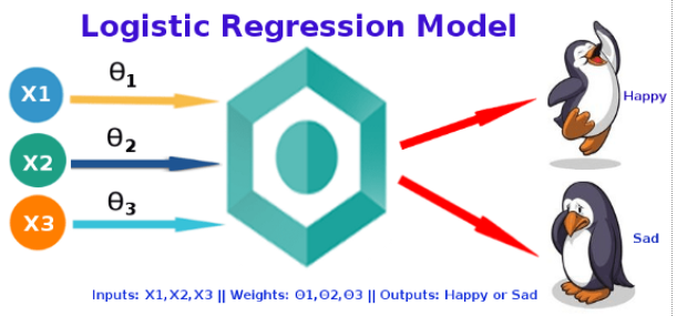
Logistic Regression was used in the biological sciences in early twentieth century. It was then used in many social science applications. Logistic Regression is used when the dependent variable(target) is categorical.
- To predict whether an email is spam (1) or (0)
- Whether the tumor is malignant (1) or not (0)
Logistic regression models the probabilities for classification problems with two possible outcomes. It's an extension of the linear regression model for classification problems
3.3 K-means Clustering
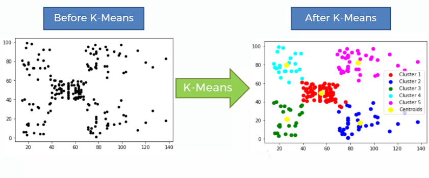
K-means clustering is one of the simplest and popular unsupervised machine learning algorithms.
The objective of K-means is simple: group similar data points together and discover underlying patterns. To achieve this objective, K-means looks for a fixed number (k) of clusters in a dataset.
A cluster refers to a collection of data points aggregated together because of certain similarities.
You’ll define a target number k, which refers to the number of centroids you need in the dataset. A centroid is the imaginary or real location representing the center of the cluster.
Every data point is allocated to each of the clusters through reducing the in-cluster sum of squares? Hm?
3.4 k-fold Cross-Validation
Lots of k's here
Cross-validation is a statistical method used to estimate the skill of machine learning models.
It is commonly used in applied machine learning to compare and select a model for a given predictive modeling problem because it is easy to understand, easy to implement, and results in skill estimates that generally have a lower bias than other methods.
Oh, so there are even methods to compare and select a model?!? Why do you even need humans for then? Let the machine face a problem, it will select the method to solve it and then solve it. Uh, even data scientists might become unecessary soon. Overexaggerating of course, but damn.